2 Blastoid Data Integration
Smart-seq2 single-cell RNA-Seq data from blastoid samples and published human embryonic datasets were integrated using the matching mutual nearest neighbors technique as implemented in fastMNN and following the protocol previously used to evaluate blastocyst-like structures via transcriptome analysis bioRxiv 2021.05.07.442980, https://github.com/zhaocheng3326/CheckBlastoids_scripts.
Read preprocessing
- Raw reads were obtained for the following data sets:
Reads were analyzed using genome sequence and gene annotation from Ensembl GRCh38 release 103 as reference. For gene expression quantification RNA-seq reads were first trimmed using trim-galore v0.6.6 and thereafter aligned to the genome using hisat2 v2.2.1. Uniquely mapping reads in genes were quantified using htseq-count v0.13.5 with parameter -s no. TPM estimates were obtained using RSEM v1.3.3 with parameter –single-cell-prior. In the case of GSE109555 data trimming and umi deduplication were performed as suggested by the authors https://github.com/WRui/Post_Implantation. For all further analyses GSE109555 of only the 3184 single cells also used in DOI: 10.1038/s41586-019-1500-0 were retained.
Loading packages and preprocessed data
suppressPackageStartupMessages({
    library(dplyr)
    library(scran)
    library(batchelor)
    library(Seurat)
    library(scales)
    library(kableExtra)
})
## import counts.all,meta.all,mt.gene,ribo.gene
load("preprocessed.E-MTAB-3929.GSE109555.Tyser2020.GSE177689.rda")table(meta.all$pj) %>%
kbl(caption = "Cells per dataset", col.names = NULL) %>%
kable_classic(full_width = F)| E-MTAB-3929 | 1529 |
| GSE109555 | 3184 |
| GSE177689 | 1595 |
| Tyser2020 | 1195 |
Filtering
For the Tyser2020 set cells with the annotation Hemogenic_Endothelial_Progenitors and Erythroblasts cells were removed as in bioRxiv 2021.05.07.442980.
For the bigger reference set GSE109555 1000 randomly sampled cells were retained.
Low quality cell were removed by keeping only cells with more than 2000 detected genes, and less than 0.125 fraction of mitochondrial genes.
Mitochondrial genes were removed from further consideration.
meta.filter <- meta.all %>%
    filter(! EML %in% c("Hemogenic_Endothelial_Progenitors","Erythroblasts")) %>%
    filter(
        !(pj == "GSE109555") |
        (pj == "GSE109555" & zhou.sample.1000 == 1)
    ) %>%
    filter(nGene > 2000 & mt.perc < 0.125)


counts.filter <- counts.all[setdiff(rownames(counts.all), mt.gene), meta.filter$cell]

table(meta.filter$pj) %>%
    kbl(caption = "Retained cells per dataset", col.names = NULL) %>%
kable_classic(full_width = F)| E-MTAB-3929 | 747 |
| GSE109555 | 1000 |
| GSE177689 | 1256 |
| Tyser2020 | 1050 |
Library normalization
Genes expressed in more than 5 cells in any dataset were used for further analysis. Scaling normalization of per-cell count data is performed using the scran deconvolution method, followed by multiBatchNorm adjustment of the size factors for systematic coverage differences. Normalized data are exported for further usage in Seurat.
experiments <- c("E-MTAB-3929","GSE177689","Tyser2020","GSE109555")

expG.set <- list()
for (b in experiments){
    temp.cell <- meta.filter %>% filter(pj==b) %>% pull(cell)
    expG.set[[b]] <- rownames(counts.filter )[rowSums(counts.filter[,temp.cell] >=1) >=5]
}
sel.expG <- unlist(expG.set) %>% unique() %>% as.vector()

sce.ob <- list()
for (b in experiments){
    temp.M <- meta.filter %>% filter(pj == b)
    temp.sce <-  SingleCellExperiment(list(counts = as.matrix(counts.filter[sel.expG,temp.M$cell])), colData = temp.M) %>%
        computeSumFactors()
    sce.ob[[b]] <- temp.sce
}

mBN.sce.ob <- multiBatchNorm(sce.ob$`E-MTAB-3929`, sce.ob$GSE177689, sce.ob$Tyser2020, sce.ob$GSE109555)
names(mBN.sce.ob) <- experiments

lognormExp.mBN <- mBN.sce.ob %>%
    lapply(function(x){logcounts(x) %>% as.data.frame()  %>% return()}) %>%
    do.call("bind_cols",.)
FastMNN
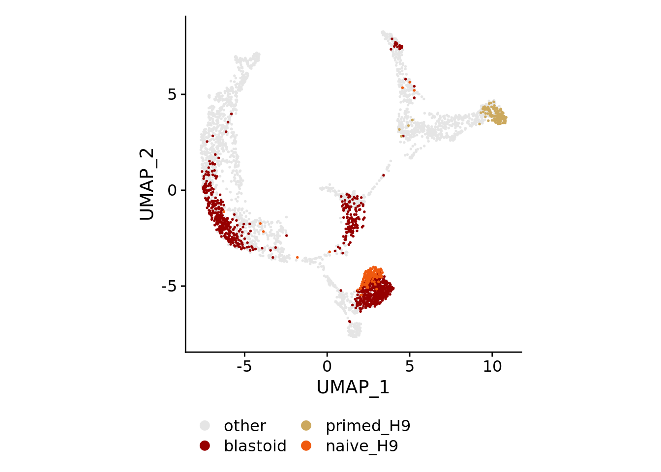
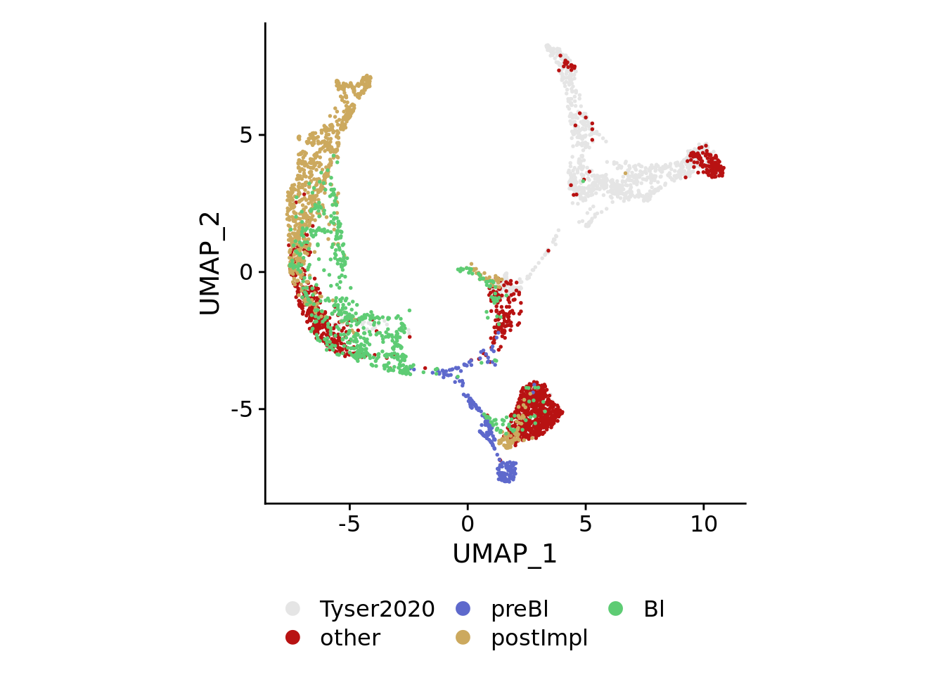
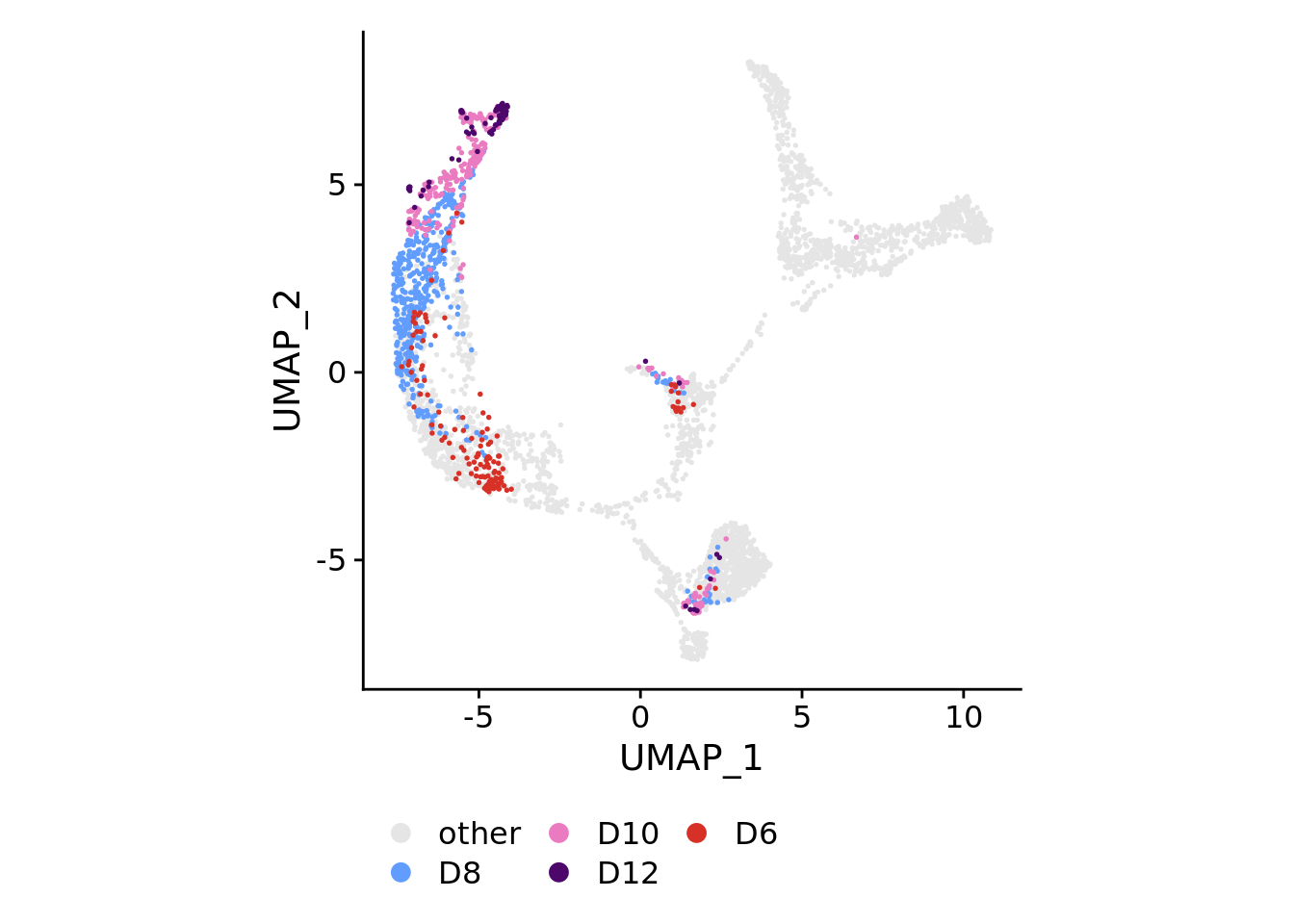
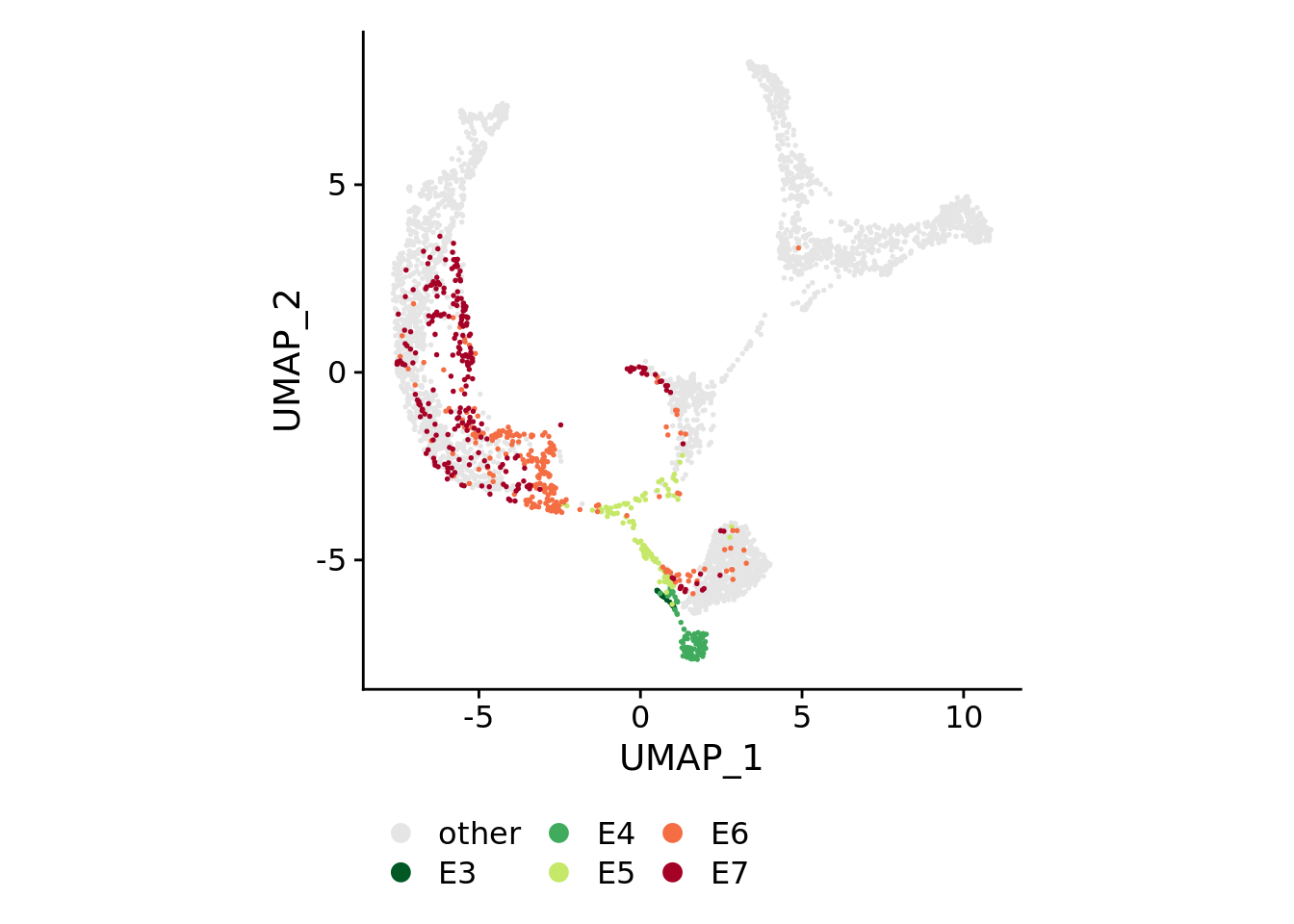
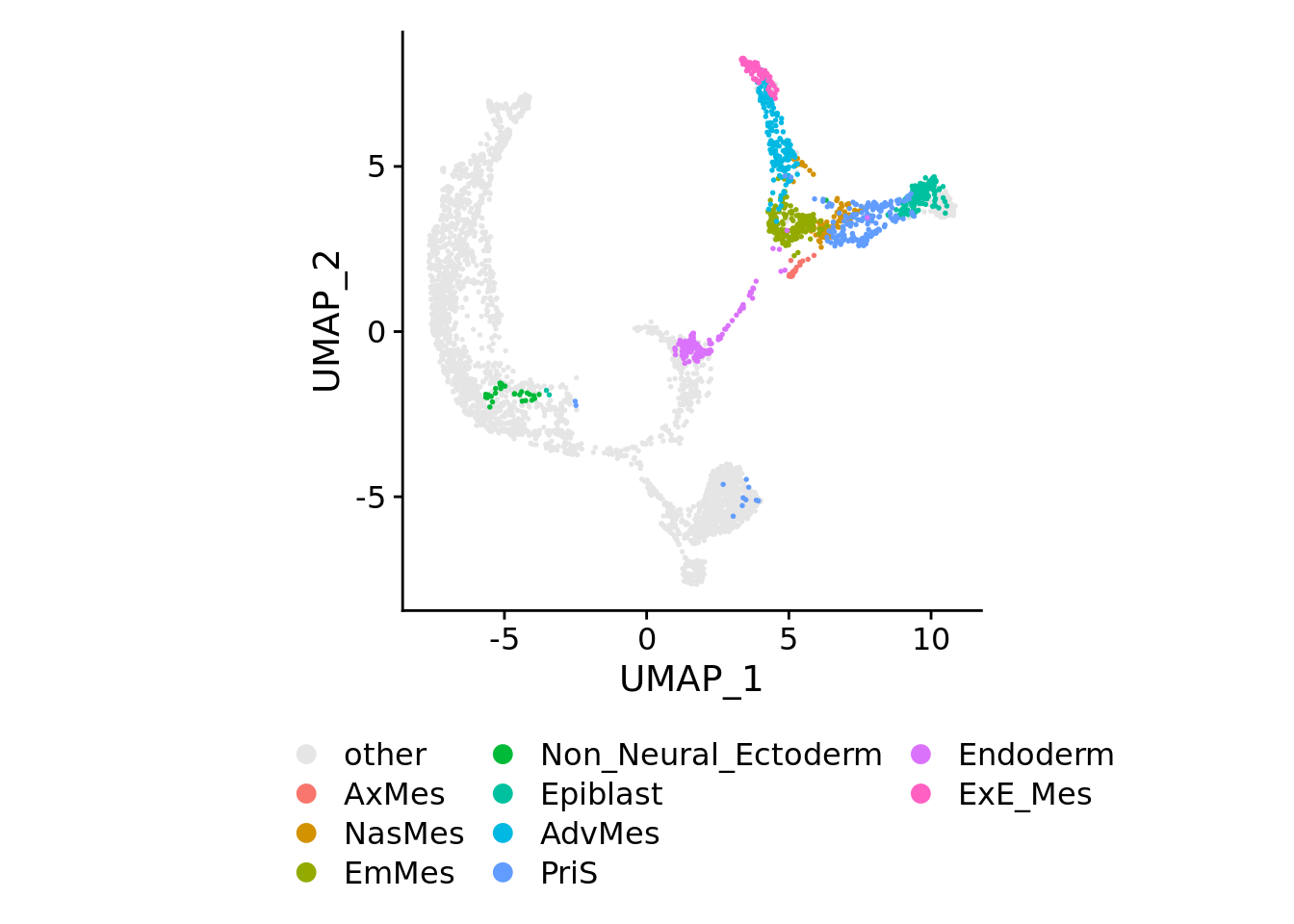
Datasets were aligned using the fastMNN approach via SeuratWrappers v0.3.0 using the log-normalized batch-adjusted expression values as input. MNN low-dimensional coordinates were than used for clustering and visualization by Uniform Manifold Approximation and Projection (UMAP).
varGene = 2000
pc = 20

sobj <-
    CreateSeuratObject(
        counts.filter[rownames(lognormExp.mBN),meta.filter$cell], meta.data = meta.filter
    ) %>%
    NormalizeData(verbose = FALSE)

sobj@assays$RNA@data <- as.matrix(lognormExp.mBN[rownames(lognormExp.mBN),colnames(sobj)])

sobj.list <- SplitObject(sobj, split.by = "pj") %>%
    lapply(function(x){ x = FindVariableFeatures(x, verbose=F, nfeatures = varGene)})
sobj.list <- sobj.list[experiments]

set.seed(123)
sobj <- SeuratWrappers::RunFastMNN(sobj.list, verbose = F, features = varGene) %>%
    RunUMAP(reduction = "mnn", dims = 1:pc, verbose = F) %>%
    FindNeighbors(reduction = "mnn", dims = 1:pc, verbose = F)

for(plotby in c("blastoid_cells","embryo_cells","zhou_time","petro_time","tyser_tissue")){
    Idents(sobj) <- plotby

    if(plotby == "blastoid_cells"){
        orderidents <- c("naive_H9","primed_H9","blastoid","other")
        cols<-rev(c("#f0590e","#cca95e","#960000","gray90"))
    } else if(plotby == "embryo_cells"){
        orderidents <- c("Bl","postImpl","preBl","CS7","other")
        cols<-rev(c("#5ecc74","#cca95e","#5e69cc","#b81212","gray90"))
    } else if(plotby == "zhou_time"){
        orderidents <- c("D6","D12","D10","D8","other")
        cols<-rev(c("#d73027","#4d076a","#ea7bc0","#619CFF","gray90"))
    } else if(plotby == "petro_time"){
        orderidents <- c("E7","E6","E5","E4","E3","other")
        cols<-rev(c("#a50026","#f46d43","#c6e868","#41ab5d","#005824","gray90"))
    }else{
        orderidents <- c(setdiff(levels(Idents(sobj)),"other"),"other")
        cols <- c("gray90", hue_pal()(length(orderidents)-1))
    }

    sobj[[plotby]] <- factor(Idents(sobj), levels = orderidents)
    ncol <- max(3, floor(length(orderidents)/6))

    print(
        DimPlot(sobj, order=orderidents, cols=cols, pt.size=0.3) +
        theme(aspect.ratio=1) +
        theme(legend.position="bottom", legend.title=element_blank()) +
        guides(color = guide_legend(override.aes=list(size=3), ncol=ncol))
    )

}
## R version 4.0.3 (2020-10-10)
## Platform: x86_64-conda-linux-gnu (64-bit)
## Running under: Debian GNU/Linux 10 (buster)
##
## Matrix products: default
## BLAS/LAPACK: /opt/conda/lib/libopenblasp-r0.3.15.so
##
## locale:
##  [1] LC_CTYPE=C.UTF-8       LC_NUMERIC=C           LC_TIME=C.UTF-8
##  [4] LC_COLLATE=C.UTF-8     LC_MONETARY=C.UTF-8    LC_MESSAGES=C.UTF-8
##  [7] LC_PAPER=C.UTF-8       LC_NAME=C              LC_ADDRESS=C
## [10] LC_TELEPHONE=C         LC_MEASUREMENT=C.UTF-8 LC_IDENTIFICATION=C
##
## attached base packages:
## [1] parallel  stats4    stats     graphics  grDevices utils     datasets
## [8] methods   base
##
## other attached packages:
##  [1] scales_1.1.1                batchelor_1.6.3
##  [3] doParallel_1.0.16           iterators_1.0.13
##  [5] foreach_1.5.1               kableExtra_1.3.4
##  [7] SeuratObject_4.0.0          Seurat_4.0.1.9013
##  [9] scran_1.18.7                SingleCellExperiment_1.12.0
## [11] SummarizedExperiment_1.20.0 Biobase_2.50.0
## [13] GenomicRanges_1.42.0        GenomeInfoDb_1.26.7
## [15] IRanges_2.24.1              S4Vectors_0.28.1
## [17] BiocGenerics_0.36.1         MatrixGenerics_1.2.1
## [19] matrixStats_0.58.0          dplyr_1.0.4
## [21] ggplot2_3.3.3               RColorBrewer_1.1-2
## [23] tidyr_1.1.2
##
## loaded via a namespace (and not attached):
##   [1] systemfonts_1.0.2         plyr_1.8.6
##   [3] igraph_1.2.6              lazyeval_0.2.2
##   [5] splines_4.0.3             BiocParallel_1.24.1
##   [7] listenv_0.8.0             scattermore_0.7
##   [9] digest_0.6.27             htmltools_0.5.1.1
##  [11] fansi_0.4.2               magrittr_2.0.1
##  [13] tensor_1.5                cluster_2.1.1
##  [15] ROCR_1.0-11               remotes_2.2.0
##  [17] limma_3.46.0              globals_0.14.0
##  [19] readr_1.4.0               svglite_1.2.3.2
##  [21] spatstat.sparse_2.0-0     colorspace_2.0-1
##  [23] rvest_1.0.0               ggrepel_0.9.1
##  [25] xfun_0.23                 crayon_1.4.1
##  [27] RCurl_1.98-1.3            jsonlite_1.7.2
##  [29] spatstat.data_2.1-0       survival_3.2-7
##  [31] zoo_1.8-8                 glue_1.4.2
##  [33] polyclip_1.10-0           gtable_0.3.0
##  [35] zlibbioc_1.36.0           XVector_0.30.0
##  [37] webshot_0.5.2             leiden_0.3.7
##  [39] DelayedArray_0.16.3       BiocSingular_1.6.0
##  [41] future.apply_1.7.0        abind_1.4-5
##  [43] pheatmap_1.0.12           DBI_1.1.1
##  [45] edgeR_3.32.1              miniUI_0.1.1.1
##  [47] Rcpp_1.0.6                viridisLite_0.4.0
##  [49] xtable_1.8-4              reticulate_1.20
##  [51] spatstat.core_1.65-5      dqrng_0.3.0
##  [53] rsvd_1.0.5                ResidualMatrix_1.0.0
##  [55] htmlwidgets_1.5.3         httr_1.4.2
##  [57] ellipsis_0.3.2            ica_1.0-2
##  [59] farver_2.1.0              pkgconfig_2.0.3
##  [61] scuttle_1.0.4             uwot_0.1.10
##  [63] deldir_0.2-10             locfit_1.5-9.4
##  [65] utf8_1.1.4                labeling_0.4.2
##  [67] tidyselect_1.1.1          rlang_0.4.11
##  [69] reshape2_1.4.4            later_1.1.0.1
##  [71] munsell_0.5.0             tools_4.0.3
##  [73] cli_2.5.0                 generics_0.1.0
##  [75] ggridges_0.5.3            evaluate_0.14
##  [77] stringr_1.4.0             fastmap_1.1.0
##  [79] goftest_1.2-2             yaml_2.2.1
##  [81] knitr_1.31                fitdistrplus_1.1-3
##  [83] purrr_0.3.4               RANN_2.6.1
##  [85] nlme_3.1-152              pbapply_1.4-3
##  [87] future_1.21.0             sparseMatrixStats_1.2.1
##  [89] mime_0.10                 xml2_1.3.2
##  [91] compiler_4.0.3            rstudioapi_0.13
##  [93] plotly_4.9.3              png_0.1-7
##  [95] spatstat.utils_2.1-0      tibble_3.0.6
##  [97] statmod_1.4.36            stringi_1.5.3
##  [99] highr_0.9                 ps_1.6.0
## [101] RSpectra_0.16-0           gdtools_0.2.3
## [103] lattice_0.20-41           bluster_1.0.0
## [105] Matrix_1.3-2              vctrs_0.3.8
## [107] pillar_1.6.1              lifecycle_1.0.0
## [109] BiocManager_1.30.10       spatstat.geom_1.65-5
## [111] lmtest_0.9-38             RcppAnnoy_0.0.18
## [113] BiocNeighbors_1.8.2       data.table_1.13.6
## [115] cowplot_1.1.1             bitops_1.0-7
## [117] irlba_2.3.3               httpuv_1.5.5
## [119] patchwork_1.1.1           R6_2.5.0
## [121] bookdown_0.22             promises_1.2.0.1
## [123] SeuratWrappers_0.3.0      KernSmooth_2.23-18
## [125] gridExtra_2.3             parallelly_1.23.0
## [127] codetools_0.2-18          MASS_7.3-53.1
## [129] assertthat_0.2.1          withr_2.4.2
## [131] sctransform_0.3.2         GenomeInfoDbData_1.2.4
## [133] mgcv_1.8-34               hms_1.0.0
## [135] rpart_4.1-15              grid_4.0.3
## [137] beachmat_2.6.4            rmarkdown_2.6
## [139] DelayedMatrixStats_1.12.3 Rtsne_0.15
## [141] shiny_1.6.0